

Since publishing Our Perspective On Market Volatility on February 29th, the market has seen wild swings in investor sentiment about the impact of COVID-19 on the economy and financial markets. Our Groundfloor asset management team has been actively engaging borrowers throughout this time to assess the risk in our portfolio, property by property and market by market.
In parallel, we have also analyzed the impact of potential adverse changes in the real estate market on Groundfloor investor portfolios. Using our full portfolio of 664 loans held by Groundfloor as of March 31, 2020 as a base, our analysis found that:
- In what many perceive as the worst-case scenario, even if housing prices decline as much as they did in 2008 (when prices dropped 22% from the peak), losses on our our portfolio would come to just 0.598% of total principal (the loss ratio), which would still deliver an overall net annualized yield of 7.1%.
- In the more likely scenario of a 5-10% reduction in price, our loss ratio would be 0.135% with a net annualized yield of 9.6% to 9.7%.
- Depending on the depth of price compression, loan repayments could be extended from 4.3 to as much as 6.2 months on average.
How is this possible, and how did our model produce these results? Dig into the details below to find out.
The Risk of Real Estate Lending
Risk takes two primary forms in real estate lending. Lenders are concerned about being repaid on time (“maturity risk”), being repaid in full (“principal risk”), and at maximum yield (“return risk"). An economic downturn or disruption to the financial system can cause distress in one or all three of these dimensions. Construction projects can encounter delays. Finished houses can sit on the market longer before selling or being refinanced. If supply far exceeds demand, or sellers face a “must-sell” situation, prices can decline.
Investors in Groundfloor LROs benefit from two key features of mortgage debt investments that limit risk relative to owning equity in a project. First, Groundfloor's security interest allows us to assume title to the property as a default remedy and an important inducement in the event of distress. Second, as a first mortgage lien holder, we have first claim on any proceeds from a sale or refinancing of the property and are the last to absorb any losses.
Groundfloor loans are underwritten with an equity cushion, which is the amount of property value in excess of the loan amount. The equity cushion provides protection for our investors as the borrower (and owner of the equity) is first in line to absorb a loss in property value. In most situations, the equity cushion is sufficient to protect investors in the loan, and the borrower absorbs any loss relative to the target property sales price.
Even surprisingly large declines in expected property value may result in little to no loss of yield for investors in Groundfloor loans. LRO investors’ yield and loan principal is only jeopardized by especially large declines in expected property value that are accompanied by an escalation of recovery expenses, such as the legal fees and carrying costs of foreclosure.
Risk Management
As a review and summary of our previous posts on the topic, proper management of these risks starts with highly professionalized underwriting policies and practices. Groundfloor loans are underwritten to a standard that ensures a significant equity cushion (typically a minimum of 30% of expected future property value, and a minimum of 10% of “as-is” property value) against decreasing home values.
Our estimate of current and future property value benefits from in-person inspection by certified appraisers, which is supplemented by data from sophisticated third-party valuation models. The appraisal and comparable properties are analyzed in detail by our in-house underwriting team to arrive at a current and future valuation of the property. Our lending criteria allow more experienced real estate entrepreneurs to borrow more in relation to property value than less experienced ones.
Following underwriting and closing, to help control risk over time, Groundfloor holds back all or substantially all of the funds needed to renovate the property. Our asset management team proactively monitors renovation progress throughout the term of the loan. Third-party inspectors verify the completion of all construction work prior to authorizing draws to pay for the associated materials and labor. When projects run into unanticipated delays, or market conditions change, we work collaboratively with borrowers while aggressively protecting our investors’ capital with the full range of legal remedies available when necessary.
The Impact of COVID-19 on the Housing Market
The primary dynamic influencing prices in the U.S. housing market over the past eight years has been, and continues to be, undersupply. According to a macroeconomic analysis by the Urban Institute, every year since 2013 the United States has supplied between 100-500 thousand fewer housing units than the market demanded. This is especially true for the starter and mid-range houses we finance.
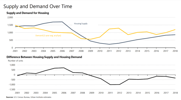
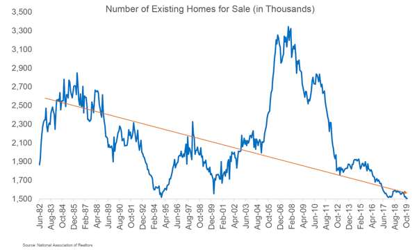
According to the National Association of Realtors, as of year-end 2019 the number of existing homes for sale dipped to the lowest level since 1995. In our view, even as demand recedes as a result of COVID-19 or other economic shocks, supply will do so as well. We believe that supply would have to exceed demand for a very long time in order to catch up to aggregate pent-up demand. Anecdotal evidence we’re hearing from borrowers and observing in April sales within our portfolio supports this view.
A deep recession and/or financial crisis in 2020 could result in temporary reductions in home prices nationally, in specific housing segments, or in local markets. In the housing crash of 2008, median home prices on a nationwide basis declined 22% from the 2007 peak to the trough in 2011:
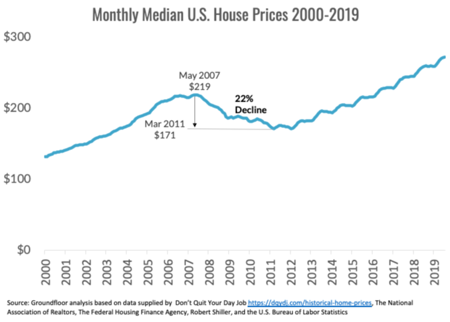
The circumstances that drove housing price inflation from the 1990s through 2007 and the subsequent decline were quite different from the market forces that have been at play since then. While price declines are always possible and we can expect to see some in 2020, beyond this year and over the long-term we feel very confident that home prices in the markets and segments we serve will either not suffer from significant price pressure, or will recover from it quickly.
Our Portfolio Stress Test
Nevertheless, despite our positive long-term view, we understand investors are concerned about the economy and its potential effect on home prices, and in turn the impact on their Groundfloor portfolios.
We are first and foremost concerned with protecting our investors’ principal. We view that risk as primary over the timing of repayment. In distressed situations, our policies and practices reflect a preference for capital to be returned late and in full, rather than on-time and with a loss. Our stress test analysis takes both priorities into account as we examine the dynamics of returning investors’ principal under different scenarios that could develop over the next six months.
We structured our stress test to model the impact to investor returns of potential price declines and increased resolution timelines, based on the current performance status and expected repayment timeline for 664 loans outstanding in our portfolio as of March 31, 2020.
Here’s the methodology we used:
- We assigned a current performance status to each loan (Performing, Sub-Performing, or Non-Performing) and extended the expected resolution period based on its status.
- Next, we calculated a projected payoff amount for each loan as of the expected resolution date, and compared the projected property value to determine the expected recovery amount.
- For every loan with an expected recovery amount that was sufficient to repay principal, but not full interest, we reduced the interest earned on that loan. For every loan with an expected recovery amount that was less than the principal balance, we subtracted the expected costs of foreclosure and recovery. We also made additional adjustments for properties that are located in jurisdictions with more expensive and time-consuming foreclosure processes versus less costly and quicker ones.
- Finally, we modeled three increasingly higher percentage declines in property sales prices (5%, 10% and 22%) across the portfolio. The changes in this variable impacted resulting average time to expected repayment based on recovery timeline, loss ratios based on an increased incidence of foreclosure, and yields based on lower total recoveries.
Our model is more conservative than what normally happens in the reality of managing distressed situations. In actual practice, we choose to avoid the costs and time required to foreclose in favor of achieving a higher return sooner by accepting a lower yield rather than risking principal loss. The model likely overstates the length of time and understates the recovery that would be actually achieved.
We’ve applied this analysis to one representative loan as an addendum to this post for those interested in a deeper dive into our methodology.
The Results
Overall, without taking potential losses into account, our current portfolio of loans is expected to yield a weighted average annualized gross return of 10.3% with an average total maturity of 11.3 months. Here are the impacts on the net loss ratio, net annualized yield, and repayment time frame based on the following declines in average home sales prices (and therefore after repair value):
| Price Decline | Loss Ratio | Net Yield | Repayment |
| 5% | 0.135% | 9.7% | +4.3 months |
| 10% | 0.135% | 9.6% | +4.7 months |
| 22% | 0.598% | 7.1% | +6.2 months |
As the table shows, even the worst-case (2008) scenario delivers a positive yield, albeit on a somewhat extended time frame. With each deeper price decline, more loans would be expected to experience principal loss, reducing the portfolio’s overall expected yield.
It is important to note that these figures are based on the entire outstanding Groundfloor portfolio, analyzed as a weighted average, which means larger loans have a larger impact. Each investor’s individual experience will differ depending on which loans they hold and how much is invested in each one. We have advocated for broad diversification before; now more than ever, being well-diversified is even more important to weather times of economic dislocation and contraction.
Addendum: An Example Loan
Loan: 800 Fayetteville Rd. SE, Atlanta, GA 30316
Origination Details:
| Origination Date | July 31, 2019 |
| Loan Amount | $276,690 |
| Construction Holdback | $83,000 |
| Interest Rate | 13.0% |
| Maturity Date | July 31, 2020 |
| As Is Value | $260,000 |
| ARV | $350,000 |
Current Status:
Payoff Amount As of May 8, 2020: $304,480
Good Standing: Yes
Stress Test Analysis:
- Since the maturity date of this loan is not after September 30, 2020, we assume that the loan will need to be extended. The current payoff amount at the time of analysis (May 8, 2020) exceeds 85% of the estimated After-Repair Value (ARV), so we set the estimated length of the resolution period to six months beyond the original maturity date (January 27, 2021).
- Next, we calculated the payoff due at the extended maturity date ($331,244) and compared that figure to a range of estimated property values to arrive at an expected recovery amount for each value. A sale at the original ARV of $350,000 would result in proceeds sufficient to afford a full recovery, providing a cushion of over $18,000 to cover transaction costs. With a 5% reduction of estimated ARV, the property would sell for $332,500; at a 10% reduction, $315,000; and at a 22% reduction $273,000.
- All price reduction scenarios for this loan resulted in payoff amounts that exceeded 95% of the ultimate sales price (e.g. the 5% priced decline of $331,244 is 99.6% of $332,500). We therefore subtracted the estimated costs of foreclosure and recovery of 7% ($24,110 to $28,725, depending on final sales price) and extended the timeline required to complete it to July 26, 2021 (six additional months beyond the original six-month extension). As noted above, if circumstances allow, we would normally choose to settle with the borrower for a reduction in interest rather than pursue foreclosure. For the purposes of this model, we assume the worst-case scenario of being forced to foreclose.
- We determined investor losses or annualized returns for each price reduction scenario taking all of the factors above into account. In the case of a 5% price compression, for example, we modeled net proceeds to investors of $304,225 (a $332,500 sales price, less $28,725), a total return of 9.95% over 776 days since origination for an annualized yield of 5.0%. A 10% price compression resulted in a 2.05% yield. Only the 22% price compression scenario resulted in a loss, in this case $27,800 (the $273,000 sales price less $24,110 in costs, yielding $248,890 compared to the principal of $276,690), a loss of 10.05%.
This same process was applied to the other 663 loans in our portfolio. Net recoveries were aggregated to generate an overall weighted average loss ratio and weighted average net yield.
Your Comments :